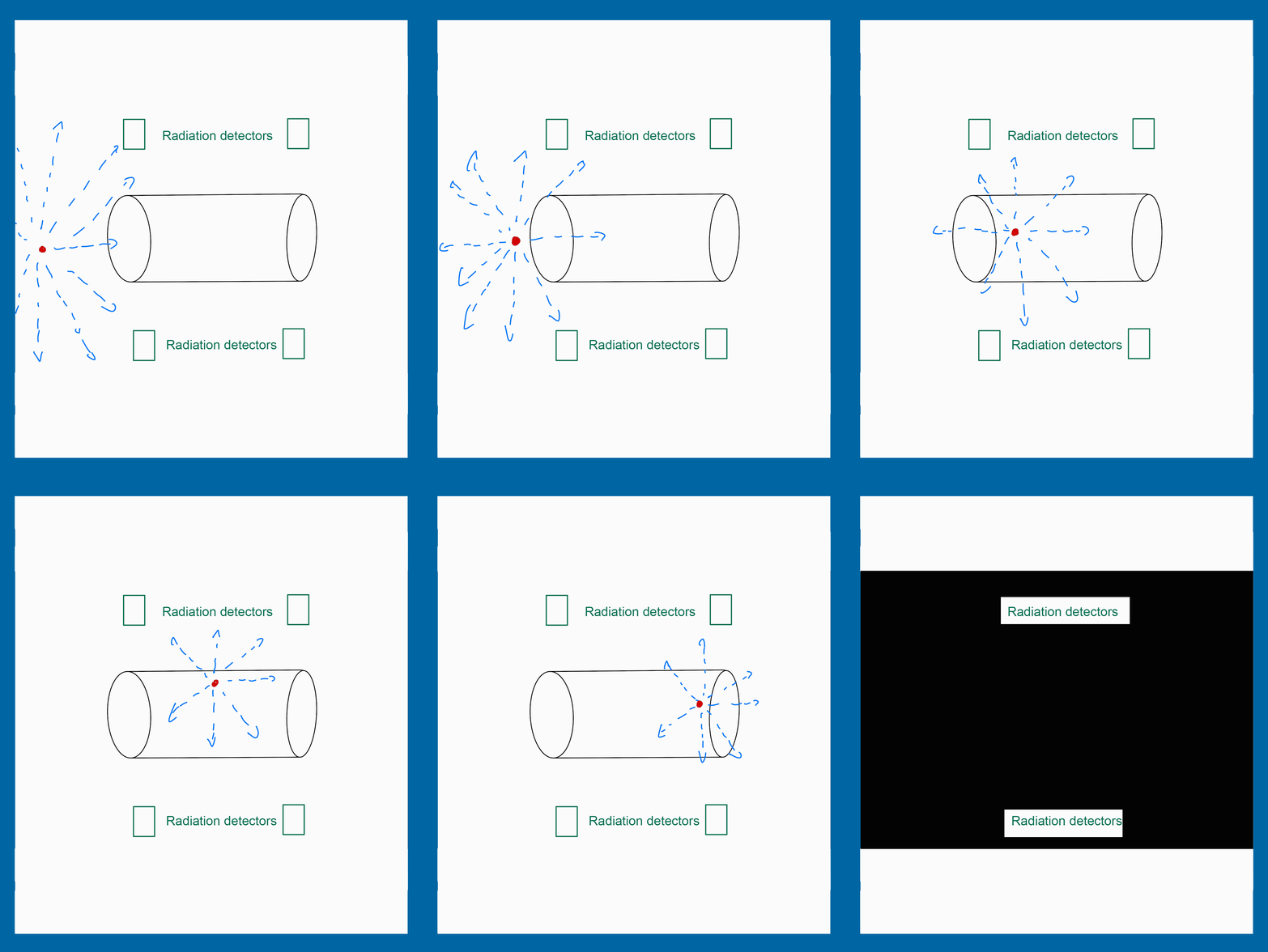
Particle moving

Particle Path Reconstruction

Introduction

Radioactive Particle Tracking (RPT) is a technique for fluid measurement which uses radiation detectors to determine the position of a radioactive source. A key stage in the deploying of the RPT is the calibration process. The calibration process intends to record the response for a known particle position and a known detector position.

The positioning of the radiation detectors can influence in the particle detection. Some position increases the number of particles detected and others have a contrary effect.

The goal of this work was evaluated which detector array gave the best quality information. To do this, an exploratory data analysis was carried out, and two machine learning algorithms with the same architecture were built and tested.

The best detector array was determined with two metrics Mean Euclidian Distance Error (MEDE). Then, the two best results were tunned the hyper-parameters of the models.
Importance of the Project
  1. Measuring properly the properties of fluids can be insigths that traditionally are not considered in the engineering.
  2. Generate algorithms is the first step to deploy for in-vivo facilities.
  3. Generate new algorithms helps to develop an own RPT system.
Data information:
  1. The data comes from the following Kaggle repository: https://github.com/sebassaras02/RPT_array_pos
  2. The data for training was 10000 positions. This data is 25 straight and 25 helicoidal trajectories.
  3. The data for test was 1000 random positions. They were only used for testing.
Exploratory Data Analysis Results
  1. Arrays 2, 3, and 4 got several zero-counting positions. A zero-counting position is a particle position where a detector is not able to collect any data.
  2. The array 3 had more around 300 zero-counting positions.
  3. The radiation detector response and particle position do not seem to have a linear correlation.
Models built

K-Nearest Neighbors Regressor

  • n_neighbors = 10
  • weigths = 'distance'

Feedforward Neural Network

  • 4 Dense Layers (1 Input, 2 Hidden, and 1 Output))
  • Each layer had a dropout of 20%.
  • Loss function was MSE, and the metric was MAE for the training stage
Final model results

    The best detector array was the number 3

  • The K-Nearest Neighbors (K-NN) Regressor and the Feedforward Neural Network a score roughly of 0.228
  • The MEDE score for the tunned models were of 0.226 for the K-NN regressor and 0.21 for the Neural Network.
  • The hyper-parameter tuning did not represented an importance enhancement of the algorithms.

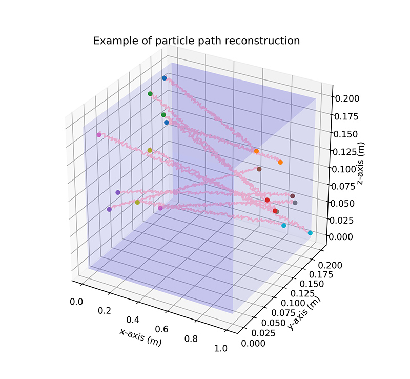
The following shows an example of how the particle path is reconstructed.

Trajectory reconstructed
Data Treatment Process
  • The data was loaded and extracted only the useful information.
  • Generation of the dataframes
  • The data was normalized with a MinMaxScaler
  • Exploratory Data Analysis
  • Models development
  • Models testing
  • Hyper-parameter tunning
  • Show code

    Sebastián

    Sarasti

    Follow me on my social media channels to know more about my projects.

    Follow Us

    Get In Touch

    Pujilí, Cotopaxi, Ecuador

    sebitas.alejo@hotmail.com

    © Sebastián Sarasti Zambonino. All Rights Reserved.

    Designed by HTML Codex

    Edited by Sebastián Sarasti and Angel Bastidas